thebookofshaders/10

Generative designs

It is not a surprise that after so much repetition and order the author is forced to bring some chaos.

Random

Randomness is a maximal expression of entropy. How can we generate randomness inside the seemingly predictable and rigid code environment?

Let's start by analyzing the following function:

Above we are extracting the fractional content of a sine wave. The sin() values that fluctuate between -1.0 and 1.0 have been chopped behind the floating point, returning all positive values between 0.0 and 1.0. We can use this effect to get some pseudo-random values by "breaking" this sine wave into smaller pieces. How? By multiplying the resultant of sin(x) by larger numbers. Go ahead and click on the function above and start adding some zeros.

By the time you get to 100000.0 ( and the equation looks like this: y = fract(sin(x)*100000.0) ) you aren't able to distinguish the sine wave any more. The granularity of the fractional part has corrupted the flow of the sine wave into pseudo-random chaos.

Controlling chaos

Using random can be hard; it is both too chaotic and sometimes not random enough. Take a look at the following graph. To make it, we are using a rand() function which is implemented exactly like we describe above.

Taking a closer look, you can see the sin() wave crest at -1.5707 and 1.5707. I bet you now understand why - it's where the maximum and minimum of the sine wave happens.

If look closely at the random distribution, you will note that the there is some concentration around the middle compared to the edges.

A while ago Pixelero published an interesting article about random distribution. I've added some of the functions he uses in the previous graph for you to play with and see how the distribution can be changed. Uncomment the functions and see what happens.

If you read Pixelero's article, it is important to keep in mind that our rand() function is a deterministic random, also known as pseudo-random. Which means for example rand(1.) is always going to return the same value. Pixelero makes reference to the ActionScript function Math.random() which is non-deterministic; every call will return a different value.

2D Random

Now that we have a better understanding of randomness, it's time to apply it in two dimensions, to both the x and y axis. For that we need a way to transform a two dimensional vector into a one dimensional floating point value. There are different ways to do this, but the dot() function is particulary helpful in this case. It returns a single float value between 0.0 and 1.0 depending on the alignment of two vectors.

Take a look at lines 13 to 15 and notice how we are comparing the vec2 st with another two dimensional vector ( vec2(12.9898,78.233)).

• Try changing the values on lines 14 and 15. See how the random pattern changes and think about what we can learn from this.

• Hook this random function to the mouse interaction (u_mouse) and time (u_time) to understand better how it works.

Using the chaos

Random in two dimensions looks a lot like TV noise, right? It's a hard raw material to use to compose images. Let's learn how to make use of it.

Our first step is to apply a grid to it; using the floor() function we will generate an integer table of cells. Take a look at the following code, especially lines 22 and 23.

After scaling the space by 10 (on line 21), we separate the integers of the coordinates from the fractional part. We are familiar with this last operation because we have been using it to subdivide a space into smaller cells that go from 0.0 to 1.0. By obtaining the integer of the coordinate we isolate a common value for a region of pixels, which will look like a single cell. Then we can use that common integer to obtain a random value for that area. Because our random function is deterministic, the random value returned will be constant for all the pixels in that cell.

Uncomment line 29 to see that we preserve the floating part of the coordinate, so we can still use that as a coordinate system to draw things inside each cell.

Combining these two values - the integer part and the fractional part of the coordinate - will allow you to mix variation and order.

Take a look at this GLSL port of the famous 10 PRINT CHR$(205.5+RND(1)); : GOTO 10 maze generator.

Here I'm using the random values of the cells to draw a line in one direction or the other using the truchetPattern() function from the previous chapter (lines 41 to 47).

You can get another interesting pattern by uncommenting the block of lines between 50 to 53, or animate the pattern by uncommenting lines 35 and 36.

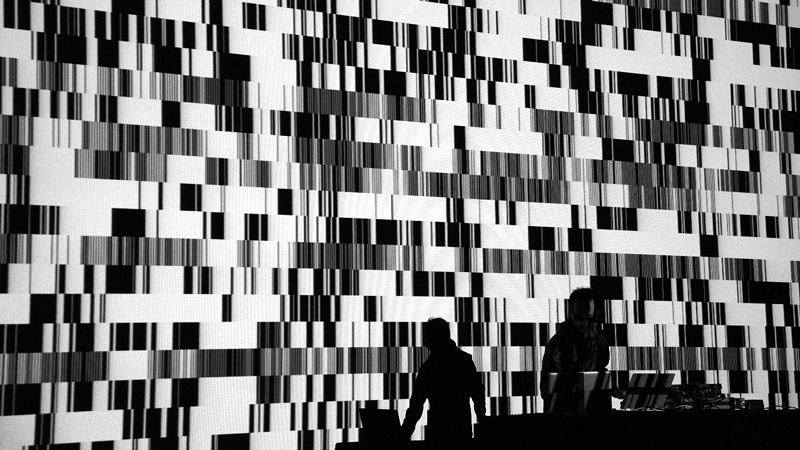
Master Random

Ryoji Ikeda, Japanese electronic composer and visual artist, has mastered the use of random; it is hard not to be touched and mesmerized by his work. His use of randomness in audio and visual mediums is forged in such a way that it is not annoying chaos but a mirror of the complexity of our technological culture.

Take a look at Ikeda's work and try the following exercises:

• Make rows of moving cells (in opposite directions) with random values. Only display the cells with brighter values. Make the velocity of the rows fluctuate over time.

• Similarly make several rows but each one with a different speed and direction. Hook the position of the mouse to the threshold of which cells to show.

• Create other interesting effects.

Using random aesthetically can be problematic, especially if you want to make natural-looking simulations. Random is simply too chaotic and very few things look random() in real life. If you look at a rain pattern or a stock chart, which are both quite random, they are nothing like the random pattern we made at the begining of this chapter. The reason? Well, random values have no correlation between them what so ever, but most natural patterns have some memory of the previous state.

In the next chapter we will learn about noise, the smooth and natural looking way of creating computational chaos.

For your toolbox

• LYGIA's generative functions are a set of reusable functions to generate patterns in GLSL. It's a great resource to learn how to use randomness and noise to create generative art. It's very granular library, designed for reusability, performance and flexibility. And it can be easily be added to any projects and frameworks.