## Color

We didn’t get the chance to talk about GLSL vectors types, so before going further is important to learn more about these variable. And the subject of colors is a great way to learn about it.
If you are familiar with object oriented programming paradigms you probalby had notice that we have been accessing the data inside the vectors like any regular C-like ```struct```.
```glsl
vec3 red = vec3(1.0,0.0,0.0);
red.x = 1.0;
red.y = 0.0;
red.z = 0.0;
```
Define color using a *x*, *y* and *z* notation can be confusing and miss leading, right? That's why there are other ways to access the same information, but with different name. The values on ```.x```, ```.y``` and ```.z``` are overloaded to ```.r```, ```.g``` and ```.b```, and to ```.s```, ```.t``` and ```.p```. Also, because vectors are essentially arrays of value you can access to the data just by using the index position of the component you want to modify or set. This diferent ways of pointing to the variables inside a vector are just nomenclatures designed to help you writing clear code. At the same time, as a lenguage helps you organize and construct sense. This flexible detail will be the door for you to think interchangalbe about colors and space coordintates.
The following lines shows al the homologous ways to access the same data:
```glsl
vec4 vector;
vector[0] = vector.r = vector.x = vector.s;
vector[1] = vector.g = vector.y = vector.t;
vector[2] = vector.b = vector.z = vector.p;
vector[3] = vector.a = vector.w = vector.q;
```
Another great feature of vectors types on GLSL is that the properties can be combined in any order you want. Making easy for example to cast and mix values. This hability is call *swizzle*.
```glsl
vec3 yellow, magenta, blue;
yellow.rg = vec2(1.0);
yellow[2] = 0.0;
magenta = yellow.rbg;
blue.b = magenta.z;
```
#### For your toolbox
If you have a background on design or new media, you are probably used to picking colors with number, which could be very counterintuitive. Lucky you, there are a lot of smart programs that make this job easy. Research for one that fits your needs and then train it to delivery colors in ```vec3``` or ```vec4``` format. For example here are the templates I use on [Spectrum](http://www.eigenlogik.com/spectrum/mac):
```
vec3({{rn}},{{gn}},{{bn}})
vec4({{rn}},{{gn}},{{bn}},1.0)
```
### Mixing color
Now that we know how colors could be define is time to integrate this with our previus knowladege. On GLSL there is a very usfull function that let you mix two values in percentages named ```mix()```. Can you imagen what's the percentage range? Yes, between values between 0.0 and 1.0! Which is perfect for you, after those long hours practicing your karate moves in the fense. Is time to use them!
Check the following code at line 18 and see how we are using the absolute values of a sin wave over time to mix ```colorA``` and ```colorB```.
Show of your skills by:
* Make an expressive transition between colors. Think on a particular emotion. What color seams the more representative of it? How it apears? how it fades away? Think on another emotion and the matching color for it? Change the begining and ending color of above code to much those emotions. Then animate the transition using shaping functions. Robert Penner develop a series of popular shaping function for computer animation popularly known as [easing functions](http://easings.net/), you can use some [this example](../edit.html#06/easing.frag) as research and inspiration, but the best result will come by making your own transitions.
### Playing with gradients
The ```mix``` function have more to offer. Instead of a single ```float``` can pass a variable type that match the two first arguments, in our case a ```vec3```. By doing that we gain control over the mixing porcentages of each individual channel.
Take a look to the following example.
Similarly to the examples on the previus chapter we are hooking the transition to the normalized *x* coordinate and visualizing it with a line. You can see how all channels goes a long together.
Now, uncoment line number 25 and see what happens. Then try the lines 26 and 27. Remember that the lines visualize the amount ```colorA``` and ```colorB``` to mix per channel.
You probably recognice the three shaping functions we are using in lines 25 to 27. Play with them! Is time for you to explore and show of your skills learned on the previus chapter and make interesting gradient. Try the following excersices:
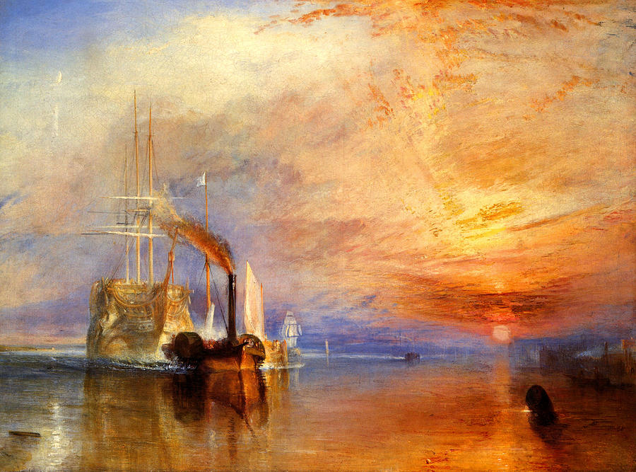
* Compose a gradient that resemblance a William Turner sunset
* Animate a transition between a sunrise and sunset using ```u_time```.
* Can you make a rainbow just using what we have learn until now?
* Using ```step()``` function create a procedural flag.
### HSB
Is hard to bring the subject of color with out speaking about color space. As you probably know there are different ways to organize color beside by red, green and blue channel.
[HSB](http://en.wikipedia.org/wiki/HSL_and_HSV) stands for Hue, Saturation and Brightness (or Value) and is a more intuitive and useful organization of colors. Take a moment to read the ```rgb2hsv()``` and ```hsv2rgb()``` functions on the following code.
Similarly to last mix example this functions plays with the interpolation of the diferent chapters to map it acording to hue.
By mapping the position on the x axis to the Hue and the brightness to the length we can obtain that nice spectrum of visible colors. This spacial distribution of color can be very handy becase, une more time, share the range between 0.0 to 1.0.
This HSB is particularly intuitive for understanding color composition, while give as extraordinary control of our values. Reason why is the default choose for color pickers user interface.
### HSB in polar coordinates
HSB was originally designed to be represented on polar coordinates (based on the angle and radius) instead of cartesian coordinates (based on x and y). To map our HSB function to polar coordinates we need to obtain the angle and distance from the center of the viewport to the fragment coordinate. For that we will use the ```atan(y,x)``` (which is the GLSL version of ```atan2(y,x)```) and the ```length()``` function.
Using vectorial and trigonometrical functions, could sound wierd in this content but ```vec2```, ```vec3``` and ```vec4``` are nothing but vectors. We will start treat colors and vectors similarly, in fact you will find very enpowering this conceptual flexibility couldbe.
If you where wondering, there are more geometric functions beside [```length```](http://www.shaderific.com/glsl-functions/#length) like: [```distance()```](http://www.shaderific.com/glsl-functions/#distance), [```dot()```](http://www.shaderific.com/glsl-functions/#dotproduct), [```cross```](http://www.shaderific.com/glsl-functions/#crossproduct), [```normalize()```](http://www.shaderific.com/glsl-functions/#normalize), [```faceforward()```](http://www.shaderific.com/glsl-functions/#faceforward), [```reflect()```](http://www.shaderific.com/glsl-functions/#reflect) and [```refract()```](http://www.shaderific.com/glsl-functions/#refract). Also GLSL have special vector relational functions such as: [```lessThan()```](http://www.shaderific.com/glsl-functions/#lessthancomparison), [```lessThanEqual()```](http://www.shaderific.com/glsl-functions/#lessthanorequalcomparison), [```greaterThan()```](http://www.shaderific.com/glsl-functions/#greaterthancomparison) and [```greaterThanEqual()```](http://www.shaderific.com/glsl-functions/#greaterthanorequalcomparison).
Once we obtain the angle and the length we need to “normalize” their values to the docile range between 0.0 to 1.0 we are used to. On line 42, ```atan(x,y)``` will return an angle in radians between -PI and PI (-3.14 to 3.14), so we need to divide this number by ```TWO_PI``` (defined on the top of the code) to get values between -0.5 to 0.5 which by a simple addition we can accommodate to the desired range of 0.0 to 1.0. The radius in other hand will return a maximum of 0.5 (because we are calculatin the distance form the center of the viewport) so we need to extend this range to it double (by multiplying by two) to get a maximum of 1.0.
As you can see, our game here is all about transforming and mapping ranges to what we want.
By this time will not be a problem to try the following excersises
* Modify the polar example to get a spinning color wheel, just like the waiting mouse icon.
* Use a shaping function together with the conversion function from HSB to RGB to expand a particular hue value and shrink the rest.

* If you look closely to the color wheel used on color pickers (see the image below) use a different spectrum acording to RYB color space. For example, the oposite color of red should be green (which is his opposite), but in our example is cyan. Can you find the way to fix that in order to look exactly like the following image?

#### Note about functions and arguments
Before jumping to the next chapter let’s stop and rewind. Go back and take look to the functions on previous examples. You will notice a ```in``` before the type of the arguments. This is a [qualifier](http://www.shaderific.com/glsl-qualifiers/#inputqualifier) and in this case specify that the variable is read only. In future examples we will see that also possible to define them variables as ```out``` or ```inout```. This last one, ```inout``` is conceptually similar to passing an argument by refernce which will five us the posibility to modify a pased variable.
```glsl
int newFunction(in vec4 aVec4, // read-only
out vec3 aVec3, // write-only
inout int aInt); // read-write
```
You may not belive it, but now we have all the elements to make cool drawings. On the next chapter we will learn how to use all the tricks we have learn to makes geometric forms by *blending* the space. Yep... *blending* the space.